
“`html
Binomial Option Pricing Model
The Binomial Option Pricing Model (BOPM) is a versatile numerical method used to value options. Unlike the Black-Scholes model, which relies on complex mathematical equations, the BOPM discretizes time into a series of intervals, creating a “binomial tree” to represent potential stock price movements. This simplicity makes it easier to understand and apply, particularly when dealing with options that have complex features, such as American-style options or options on dividend-paying stocks.
How the Model Works
The core principle is that the underlying asset’s price can either go up or down during each time period. The magnitude of these upward and downward movements is determined by the volatility of the underlying asset. Let’s break it down:
- Time Steps: The lifespan of the option is divided into a number of discrete time intervals. The more intervals used, the more accurate the model becomes, but also the more computationally intensive.
- Up and Down Factors: The model calculates an ‘up’ factor (u) and a ‘down’ factor (d). ‘u’ represents the factor by which the stock price increases, and ‘d’ represents the factor by which the stock price decreases. These factors are usually derived from the volatility of the underlying asset and the length of each time period. Common formulas are: u = e^(σ√Δt) and d = 1/u, where σ is the volatility and Δt is the length of the time step.
- Risk-Neutral Probability: The model uses a risk-neutral probability (p) to calculate the expected payoff at each node of the tree. This probability isn’t a forecast of actual market movements, but rather a theoretical probability that allows us to discount the future value back to the present value without requiring a risk premium. The risk-neutral probability is calculated as: p = (e^(rΔt) – d) / (u – d), where ‘r’ is the risk-free interest rate.
- Constructing the Tree: Starting from the current stock price, the tree is built forward. At each node, the stock price either goes up (multiplied by ‘u’) or down (multiplied by ‘d’). This process is repeated for each time step until the expiration date of the option.
- Calculating Option Values at Expiration: At the end of the tree (the expiration date), the value of the option is simply its intrinsic value (the payoff). For a call option, this is max(0, Stock Price – Strike Price), and for a put option, it’s max(0, Strike Price – Stock Price).
- Working Backwards: The option values are then calculated backward through the tree, using the risk-neutral probability and discounting. At each node, the option value is the discounted expected value of the option values in the next time period. For American-style options, at each node, we also compare this calculated value with the immediate exercise value and take the higher of the two (because American options can be exercised at any time).
Advantages and Disadvantages
Advantages:
- Handles American-style options easily.
- Can be adapted to incorporate dividends and other complex option features.
- Relatively easy to understand and implement.
Disadvantages:
- Can be computationally intensive for a large number of time steps.
- Assumes constant volatility, which may not be realistic.
- Less precise than some other models, especially for European-style options when volatility is relatively stable.
Conclusion
The Binomial Option Pricing Model offers a valuable and intuitive framework for valuing options, especially when dealing with complexities that the Black-Scholes model struggles with. While it has limitations, its adaptability and ease of understanding make it a popular choice in finance.
“`
 1415×816 reading startups real options valuing sell from vlp.teju-finance.com
  547×742 reading startups real options binomial trees introduction teju from vlp.teju-finance.com
 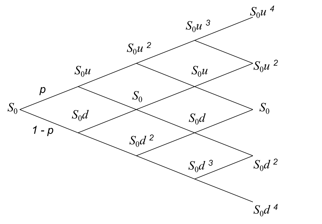 1094×761 constructing binomial tree describe stock price movement from financetrain.com
  1280×720 binomial interest rate trees spreadsheet ryan oconnell cfa from ryanoconnellfinance.com
  960×720 telecharger arbre binomial option gratuit pdfprofcom from pdfprof.com
  800×600 binomial trees from courses.cs.washington.edu
  0 x 0 binomial tree step european put option youtube from www.youtube.com
  0 x 0 binomial tree price option part youtube from www.youtube.com
  502×469 matlabtrading from www.matlabtrading.com
  1024×682 binomial trees learnsignal from www.learnsignal.com
  1024×768 chapter futures options from slideplayer.com
  1024×768 binomial tree adapted kevin wayne bk bk from slideplayer.com
  212×300 binomial tree model convertible bond pricing edhec risk climate from climateimpact.edhec.edu
  1024×768 options stock indices currencies futures from slideplayer.com
  640×640 binomial tree interest rates unit scientific diagram from www.researchgate.net
  1024×768 advanced finance black scholes from slideplayer.com
  850×1280 option pricer binomial trees home from adrian.ng
  850×752 adjusted binomial tree abandon option scientific from www.researchgate.net
  1280×675 binomial tree awesomefintech blog from www.awesomefintech.com
  474×474 variables binomial tree analysis scientific diagram from www.researchgate.net
  455×179 binomial trees learning data structures programming from rkgiitbh.github.io